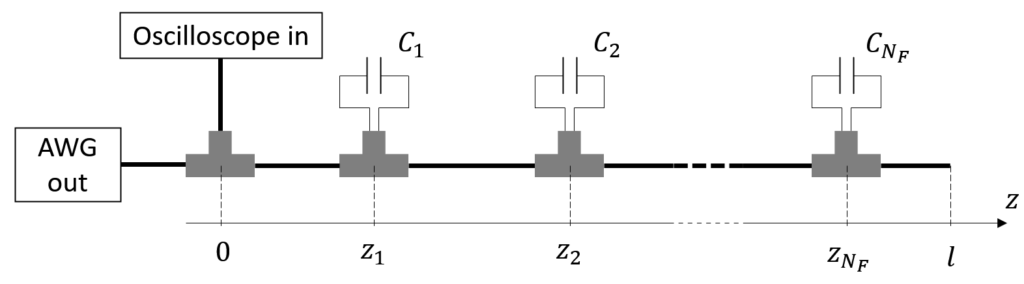
Methodology: The situation considered is represented in Fig. 1. The cable has total length  and contains  localized faults, simulated by means of capacitors connected in parallel by means of T-junctions. The capacitors are placed at a distance  from the beginning of the cable and have capacitance . The stimulus signal is generated by an Agilent 33250A AWG, while the TDR signals are acquired using a LeCroy Waverunner-2 LT262 oscilloscope. A Gaussian pulse is used as the stimulus signal.

The neural network employed was inspired by single-shot CNNs (YOLOs) for object detection. These neural networks consist of a sequence of convolutional and pooling layers. Since in the present case signals are processed in the time domain, 1D convolutional layers are used, rather than 2D ones, as the basic component of the model. The input of the first layer is the measured TDR signal, the output of the last layer is an  matrix ( is number of cells into which the length of the line is divided), which identifies position, class, impedance and probability of the fault.

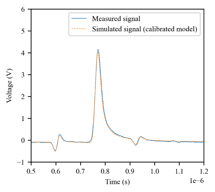
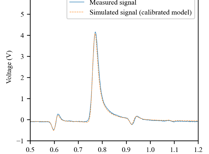
The training set of the neural network is obtained by generating simulated reflectograms under various fault conditions. The simulator uses the primary RCGL parameters of the line, which were identified using the stepped-frequency waveform reflectometry (SFWR) developed in [3]. This technique can be used easily for long cables and using low-cost, portable instrumentation. The identification obtained is quite accurate, as shown in Fig. 2.

Results: Tables I and II summarize some of the results obtained. In particular, Table I reports some results obtained on cables with four capacitive faults and shows the remarkable accuracy with which they are localized. The quantification may appear less accurate; however, it must be said that the capacities reported are simply nominal capacities of the capacitors used to simulate the fault. These capacities have quite high tolerances per se and are not related to the frequency range of the TDR signal used in the test. Table II reports statistics on the overall measurement errors in all the experiments conducted (six with a single failure, six with two failures, two with three failures, two with four failures), in terms of RMS error and mean absolute percentage error (MAPE).

Conclusions: The experiments showed that the proposed method is remarkably accurate, as well as being very general. It can be applied to the localization and characterization not only of faults in cables, but also of points of discontinuity in distributed sensitive elements.

References:

[1] Scarpetta, M.; Spadavecchia, M.; Adamo, F.; Ragolia, M.A.; Giaquinto, N. Detection and Characterization of Multiple Discontinuities in Cables with Time-Domain Reflectometry and Convolutional Neural Networks. Sensors 2021, 21, 8032. doi: 10.3390/s21238032 .

[2] M. Scarpetta, M. Spadavecchia, G. Andria, M. A. Ragolia and N. Giaquinto, “Analysis of TDR Signals with Convolutional Neural Networks,” 2021 IEEE International Instrumentation and Measurement Technology Conference (I2MTC), 2021, pp. 1-6, doi: 10.1109/I2MTC50364.2021.9460009.

[3] N. Giaquinto, M. Scarpetta and M. Spadavecchia, “Algorithms for Locating and Characterizing Cable Faults via Stepped-Frequency Waveform Reflectometry,” in IEEE Transactions on Instrumentation and Measurement, vol. 69, no. 9, pp. 7271-7280, Sept. 2020, doi: 10.1109/TIM.2020.2974110..

 

Table I. Estimation results for real cables with four capacitive faults.

	Experiment 1		Experiment 2
	Nominal	Estimated	Nominal	Estimated
Length of the cable (m)	143	142.96	143	142.96
Position of fault 1 (m)	50	49.87	50	49.88
Position of fault 2 (m)	65	65.12	65	65.03
Position of fault 3 (m)	115	114.93	115	114.95
Position of fault 4 (m)	131	131.40	131	131.32
Capacity of fault 1 (pF)	107	117	107	115
Capacity of fault 2 (pF)	217	214	152	165
Capacity of fault 3 (pF)	404	436	309	323
Capacity of fault 4 (pF)	450	441	450	439

 

Table II. Estimation errors obtained for experimental signals.

Cable length error			Fault position error				Fault capacity error
RMSE (m)	MAPE		RMSE (m)		MAPE		RMSE (pF)		MAPE
0.12		0.10%		0.13		0.22%		14		4.3%